MS Excel Vlookup and Wildcards partial text match

Use Excel Vlookup to find matching value on the basis of partial information e.g. incomplete names, beginning or even end of text characters:

MS Excel Vlookup and Wildcards partial text match: Microsoft Excel has the function of Wildcards which helps in searching for certain text string or character within vlookup function. Below are the two wildcards in MS Excel:
1) * or Asterisk: it is used after a text string to denote that any match within the vlookup range is acceptable if exactly as before the asterisk. The text string within quotes “Jim*” will search for the text beginning with the 3 alphabets if found in the same sequence at the beginning of the text. Because the wildcard * tells excel to look for a string of characters as “Jim”. Similarly, excel Vlookup will also look for all the words containing these three characters as text strings.
Note: If * asterisk is placed after the text string then it will look for the words beginning with “Jim” but if we want it to search for the specific string found anywhere within the word or text, we should used asterisk both before and after the search string i.e. *Jim*.

MS Excel Vlookup and Wildcards partial text match

2) ? or Question Mark: It will look for the specific single character mentioned before the “?” sign.
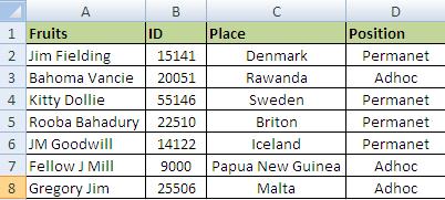
Example: Assume that on the basis of above table we are to segregate the employee names that contain the word “Jim”. We can perform this step by step action to obtain the required names using Excel VlookUp and Wildcards:
Step 1) we should write the text string in a text cell separately as depicted below:

Note: we have added the asterisk right after the text string to turn it into a wildcard in Excel.
Step 2) Create the table where data is to be fetched:

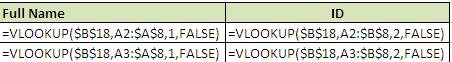
Step 3) write the formula as follows: =VLOOKUP ($B$18, $A$2:$A$8, 1, FALSE)
The below table shows the formula:

Breaking down the formula in small fragments for understanding:
=Vlookup(
It begins the formula.
Lookup value=*Jim*
Lookup Range= A2:A8.(Note: we have used “$” to lock the cells to A8, the end of table range.
Column =1 for Full Name and Column=2 for ID
We have selected “False” because we need exact match.

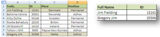
The above formula would yield us the following result:

Please note that we have got information for the highlighted cells only; the perfect functioning of wildcards within MS Excel.